Directional Light
I have used the Point-Light as a base for the Directional Light. The implementation can be found
in directional_light.cpp. The new Emitter takes two parameters: A
Color3f radiance and a Vector3f direction.
Validation
To validate the implementation, I created equal scenes for Mitsuba an compared the results.


When evaluating the emitter the radiance is returned:
                    virtual Color3f eval(const EmitterQueryRecord & lRec) const override {
                        return m_radiance;
                    }
For the following, we can think of the directional light as an infinitely big plane at an infinit distance. The most important thing here is setting the shadow-ray, to not intersect anything the negative direction of the emitted light (in the segment from the intersection until infinity).
                    virtual Color3f sample(EmitterQueryRecord & lRec, const Point2f & sample) const override {
                        lRec.p = Point3f(INFINITY);
                        lRec.pdf = 1;
                        lRec.wi = -m_direction.normalized();
                        lRec.shadowRay = Ray3f(lRec.ref, lRec.wi, Epsilon, INFINITY);
                        return m_radiance;
                    }
The likelyhood of sampling the emitter at the selected point is 1, as we will always sample the same point on the emitter.
                    virtual float pdf(const EmitterQueryRecord &lRec) const override {
                        return  1;
                    }
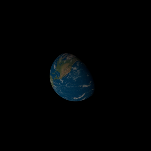
Images as Textures
I have used the checkerboard texture as a base for image textures. The implementation can be
found in image_texture.cpp. The new Emitter takes one parameter: A
String image_path which points to a jpg-texture relative to the path of the
scene.
The texture is loaded into memory when the scene is initialized. Herefore stb_image.h is used.
                        ImageTexture::ImageTexture(const PropertyList &props) {

                            filesystem::path filename = getFileResolver()->resolve(props.getString("image_path"));
                            m_image_path = filename.str();
                            int x, y, n;
                            unsigned char *data = stbi_load(m_image_path.c_str(), &x, &y, &n, 3);
                            if (data == NULL) {
                                cout << "NO IMAGE DATA HAS BEEN LOADED!" << endl;
                            }
                            else {
                                m_image_size = Vector2i(x, y);
                                m_image = std::vector>(x, std::vector(y, Color3f(0)));
                                for (int i = 0; i < x; i++) {
                                    for (int j = 0; j < y; j++) {
                                        float r = data[(j*x + i) * 3] / 254.f;
                                        float g = data[(j*x + i) * 3 + 1] / 254.f;
                                        float b = data[(j*x + i) * 3 + 2] / 254.f;
                                        m_image[i][j] = Color3f(r, g, b).pow(2.2);
                                    }
                                }

                                stbi_image_free(data);
                            }
                        }

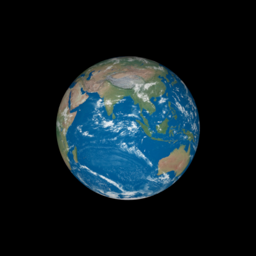
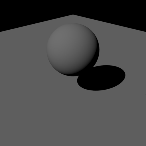
Here are the results for an analytic sphere. The results vary slightly due to different UV-mappings.
When I use a mesh the results are correct. I have used Meshlab to create the vertext normals.
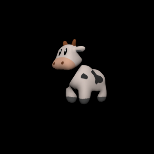
Bump Mapping
For this task, I extended two files to directly perturb the normals of the mesh. This allows the normal mapping to work with all materials without having to change all of them. Within a mesh, one can now define a String bumpmap which points to the jpg-file of a Bump-Map. In obj.cpp the Bump-Map is then stored in memory as for the image texture. Additionally, the RGB-Space is mapped to the Normal-Space.
                            float n_x = (data[(j*x + i) * 3] *2.f) - 1.f;
							float n_y = (data[(j*x + i) * 3 + 1] *2.f) - 1.f;
							float n_z = (data[(j*x + i) * 3 + 2] *2.f) - 1.f;
							bump_map[i][j] = Vector3f(n_x, n_y, n_z).normalized();
                        int x = mod(its.uv.x()*bump_map_size.x(), bump_map_size.x());
                        int y = mod(-its.uv.y()*bump_map_size.y(), bump_map_size.y());
                        Vector3f bump_normal = bump_map[x][y];

                        Point3f deltaPos1 = p1 - p0;
                        Point3f deltaPos2 = p2 - p0;
                        Point2f deltaUV1 = m_UV.col(idx1) - m_UV.col(idx0);
                        Point2f deltaUV2 = m_UV.col(idx2) - m_UV.col(idx0);

                        float r = 1.0f / (deltaUV1.x() * deltaUV2.y() - deltaUV1.y() * deltaUV2.x());
                        Vector3f dpdu = (deltaPos1 * deltaUV2.y() - deltaPos2 * deltaUV1.y())*r;

                        Normal3f n = bump_normal;
                        n = its.geoFrame.toWorld(n).normalized();
                        Vector3f s = (dpdu - n * n.dot(dpdu)).normalized();
                        Vector3f t = n.cross(s).normalized();

                        its.shFrame = Frame(s, t, n);
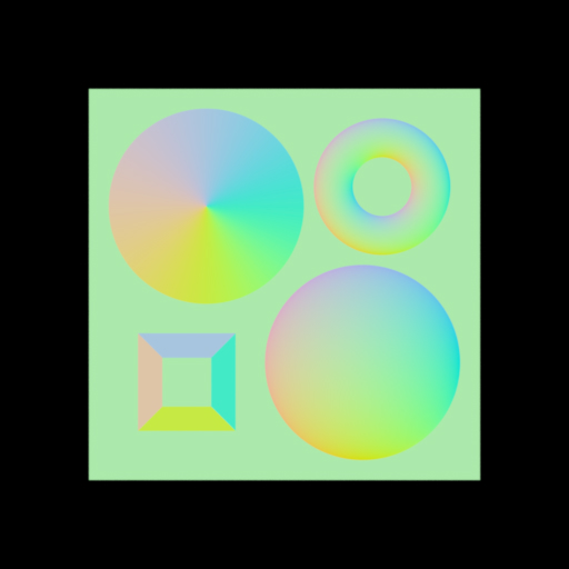
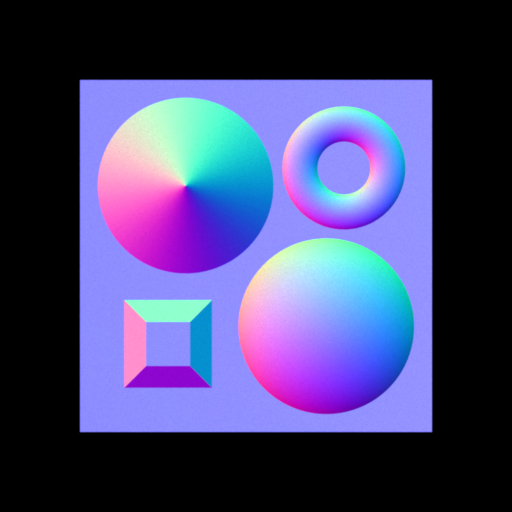
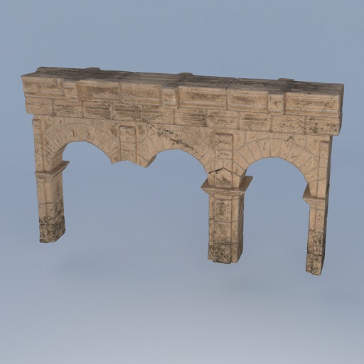
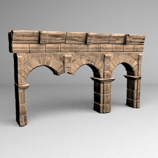
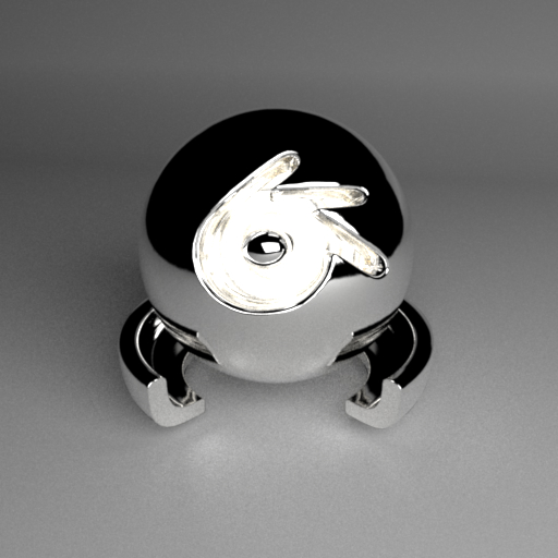
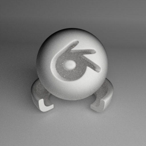
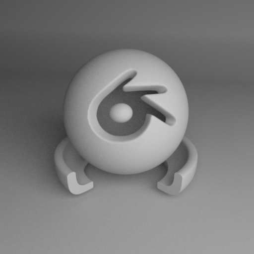
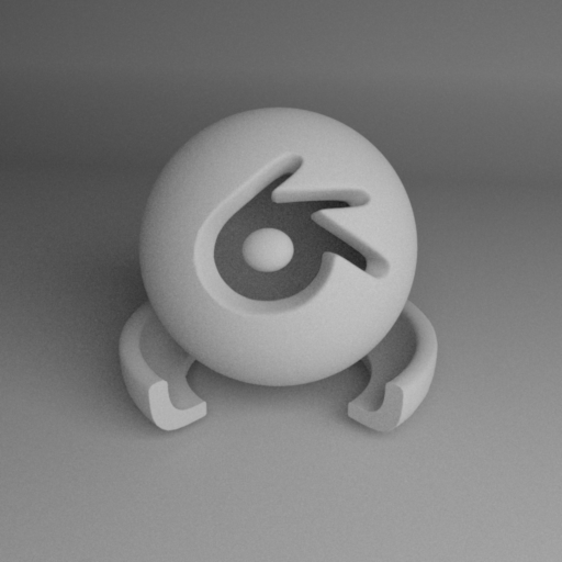
Validation
Validation of this feature was harder than anticipated. Mitsuba has a normalmap-BSDF, but it apparently only works with HDR normal maps, is not documented and tends to black out regions of the mesh for SDR normal maps. So I decided not to rely on it for validation. Using the Normal-Integrator from the first exercise, we can see that the normals are perturbed correctly. I also rendered a second scene, for which I render a comparison in blender. Here as well, the results look visually correct.
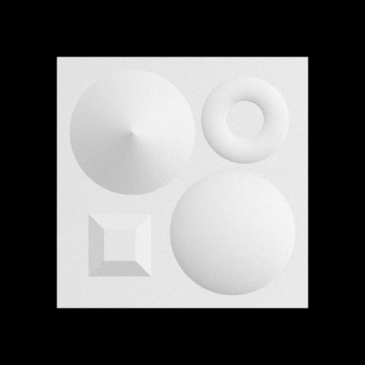
Rough conductor BSDF
For the Rough conductor in rough_conductor.cpp I used the Dielectic BSDF as a base. I then copied the evalBeckmann and smithBeckmannG1 implementations from the microfacet BSDF. As input the user can specify three values: Color3f eta and Color3f k which describe the material in the RGB-specturm and float alpha which defines the roughness. Like in Mitsuba, low alpha-values lead to a smooth surface, while higher values result in rough surface approximations. In the sample function we first sample Beckmann. The PDF is then computed to perform a sanity-check. Finally, eval(bRec) and pdf(bRec) are called.
                            virtual Color3f sample(BSDFQueryRecord &bRec, const Point2f &sample) const override {
                                Normal3f m = Warp::squareToBeckmann(sample, m_alpha);

                                float p = Warp::squareToBeckmannPdf(m, m_alpha);
                                if (p == 0)
                                    return Color3f(0.0f);

                                bRec.wo = (2.f * m.dot(bRec.wi) * m - bRec.wi);
                                return eval(bRec) * Frame::cosTheta(bRec.wo) / pdf(bRec);
                            }
Validation
To validate the implementation, I created equal scenes for Mitsuba and compared the results.


Rough Diffuse BSDF
For the Rough Diffuse BSDF in rough_diffuse.cpp I used the Diffuse BSDF as a base. As input the user can specify two values: Texture albedo, which can be both an image or a Color value and float alpha, which defines the roughness. Like in Mitsuba, low alpha-values lead to a smooth surface, while higher values result in rough surface approximations. I use the same conversion as is used in Mitsuba to make the alpha-value comparable with the alpha-value of the rough conductor.
float sigma = m_alpha / sqrt(2.f);
                        virtual Color3f sample(BSDFQueryRecord &bRec, const Point2f &sample) const override {

                            bRec.measure = ESolidAngle;
                            bRec.wo = Warp::squareToCosineHemisphere(sample);
                            bRec.eta = 1.0f;

                            return eval(bRec) * Frame::cosTheta(bRec.wo) / pdf(bRec);
                        }
Validation
To validate the implementation, I created equal scenes for Mitsuba and compared the results.


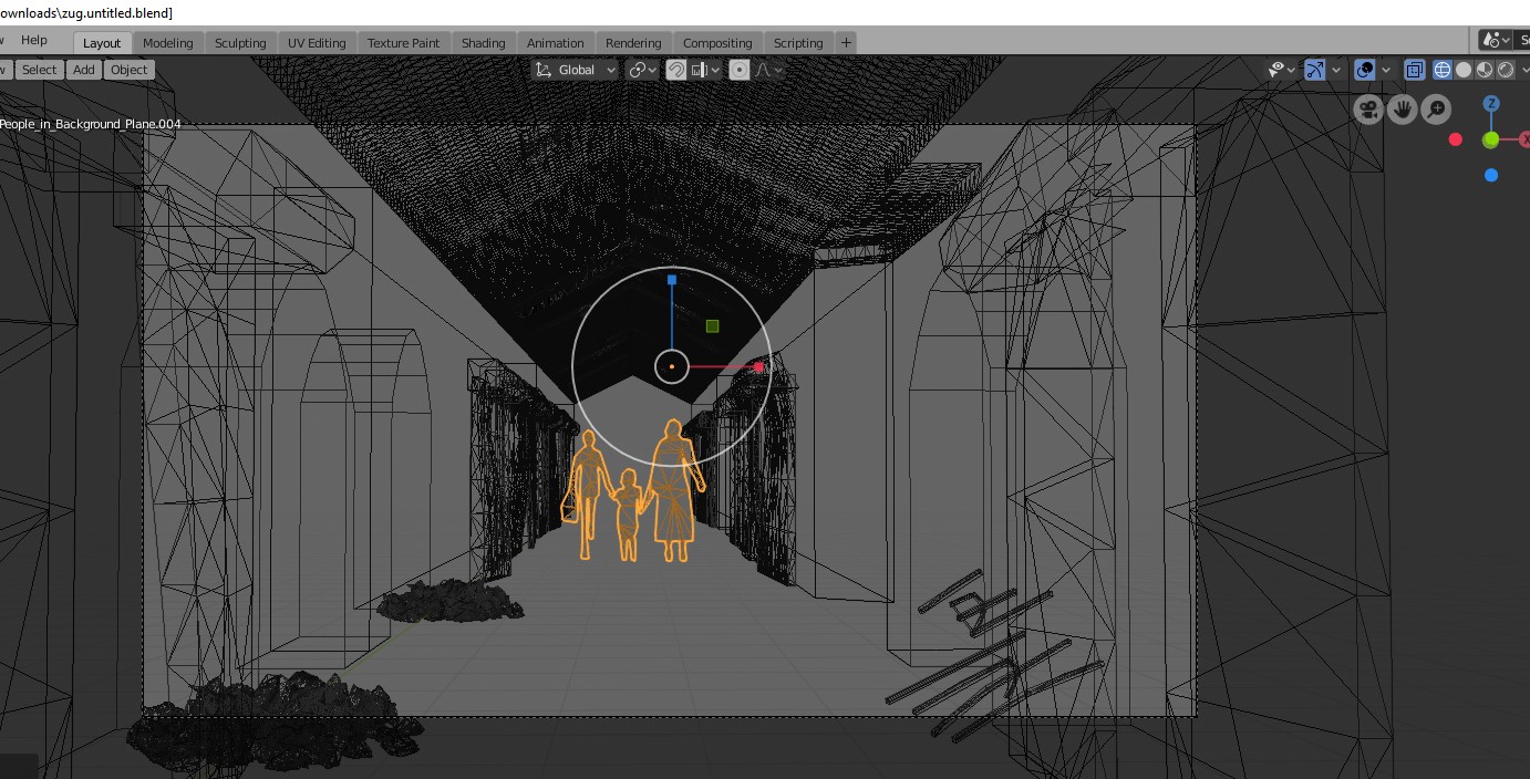
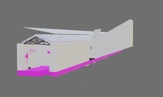
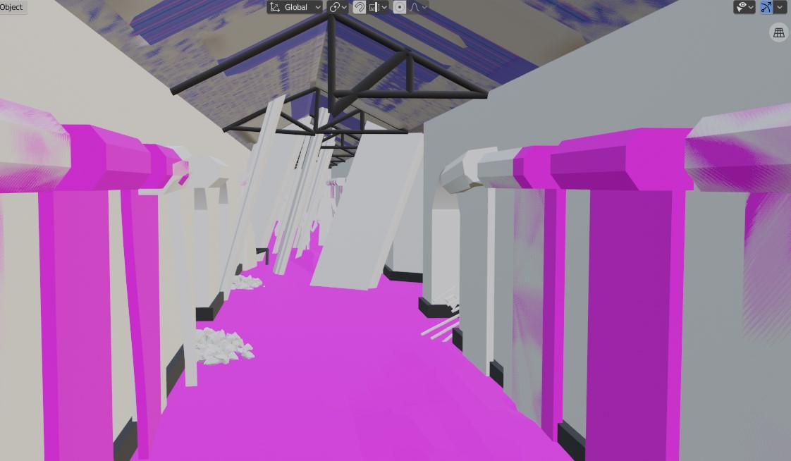
Mesh Editing
For the mesh editing, I mainly used blender and Meshlab. Aditionally, I used Adobe Photoshop to change some textures and normalmaps.